In the first part of this post I will construct four time series plots on the same graph and in the second part I will choose a nice palette for a bivariate normal density estimate. The data set for the time series plot is the Broadway show from https://think.cs.vt.edu/corgis/csv/broadway/broadway.html and the data for the bivariate normal denstiy estimate is simulated.

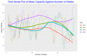
In the time series plot above we plot the mean Capacity as a function of week number, comparing years from 2010 to 2013. The choices help to distinctively distinguish the series for each year. A loess curve is overlayed on each year’s series. At the beginning of 2010 the mean capacity was 82.5, this decreased from the first week till the 13th week and then increases till the 30th week and also decreased from there till the 52nd week recording a mean capacity of about 71. In 2011 mean capacity decreased from the first week till the 9th week and increased till the 32nd week. 2012 shows a similar pattern as 2010. 2013 was interesting to look at, mean capacity increased from the first week till about the 25th week then decreased till about the 38th week and increased till the end of the year.

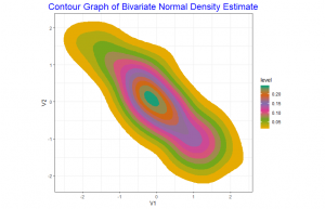
In the contour graph of the bivariate normal density estimate we use the palette “Dark2”. With this we are able to see clearly each of the contour curves well. The contour curves are ellipses. The negative slope of the major axis shows the negative correlation between the two variables and its eccentricity shows the correlation value is close to -1.