Jianing Min's MATH 6820 Blog

Loess

First, simulates some (x, y) data where the true signal follows one of the curves sin(x)+cos(x), sin(x)-cos(x), sin(x)*cos(x), .28-.88*x-0.03*x^2+.14*x^3.

Then we get a list, where d$x is the x values and d$y contains the y values.

> head(cbind(d$x,d$y))
          [,1]       [,2]
[1,] -3.141593 -0.7723653
[2,] -3.110019 -1.0347078
[3,] -3.078445 -1.3321508
[4,] -3.046871 -1.9027887
[5,] -3.015297 -1.4537965
[6,] -2.983724 -1.9512365

Using the simulated data …

1.  Construct a scatterplot of your data and overlay a lowess smooth (using the default value of f in the lowess function).

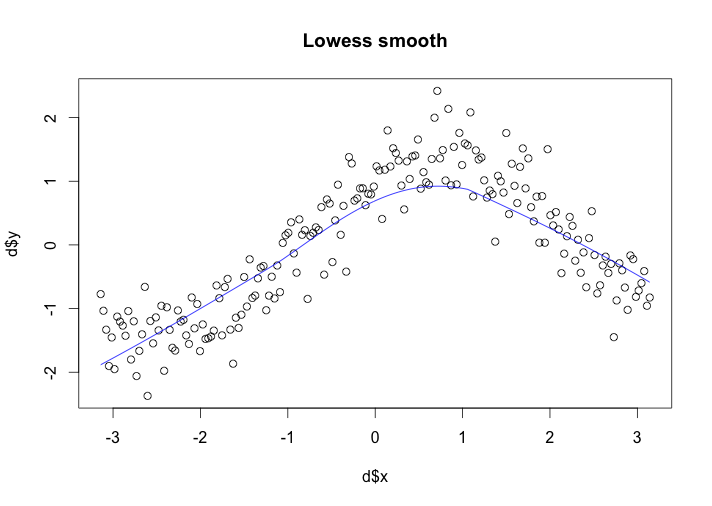
Loess produces smoothed values at any desired collection of values along the x scale and summarizes how y depends on x. From the above graph, we can see that there is nonlinear relationship between x and y. An increase in Y as x increases until x is close to 1,saying a positive relationship between x and y and the effect is nearly linear and the slope is close to 1. From 1 and above, the an decrease in Y as x increases until x is close to 3,saying a negative relationship between x and y and the effect is nearly linear and the slope is close to -1.(The whole graph is definitely nonlinear, just for better explanation, I divided the graph into two parts, each part seems linear relationship between x and y.  )

2.  Construct a plot of residuals and comment if the lowess curve has effectively found the signal.

 

 

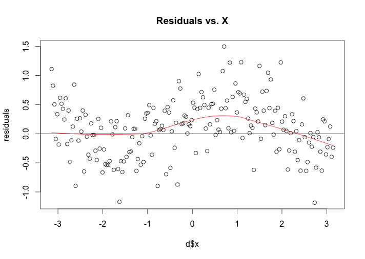
There is a fluctuant pattern in the residual graph, the problem is that the loess smoothing in the top panel has missed part of the pattern because  is too large, and this missed part has gone into the residuals. In this case, we should reduce  value, (For example, drop from default alpha to alpha=0.25 ), Although the amount of smoothing for the curve may be not great, the loess curve on the residual will be reasonable close to a horizontal line, which suggests the loess curve with  is not distorting the underlying pattern in the data.

Then I combine two graphs in one for better visual effect:

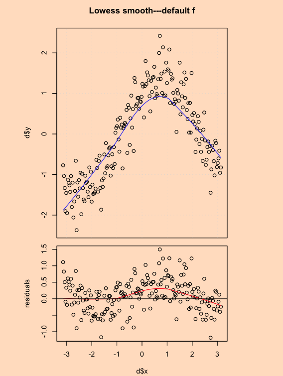 By combining two graph together, we can see clearly both relationships of y and x and residuals and x, with the same horizontal scale.

3.  Assuming that a better smooth can be found, construct a scatterplot using a better choice of f.  By the use of a residual plot, demonstrate that your choice of f is better than the default choice in 1.

Since the default f yields certain pattern in residuals, which means alphais too big, I reduce the alpha value from default to 0.25 eventually. First I tried alpha=0.5, however the loess curve on the residual graph still shows a fluctuated pattern, then I continuous drop alpha value from 0.5 to 0.4, 0.3, 0.25, until the  loess curve on the residual graph is nearly a horizontal line since the residuals should be variation in  y not explainable by x. Meanwhile, to keep alpha from being too small is to increase it to point where the residual graph just begins to show a pattern, and then use a slightly smaller value of . In this case, we can either avoid the loess curve on the residual has a pattern, or keep  from being too small. As saying above, I end up with using alpha=0.25, which make the  loess curve on the residual graph is nearly a horizontal line.

To demonstrate the whole procesure, I first upload a graph with alpha=0.5, which makes the residuals vs. X still has a certain pattern. 

From this graph, we can see that f=0.5 is not the best choice, since the fluctuated pattern still exist. Then I continuous reduce f value until the  loess curve on the residual graph is nearly a horizontal line, with f=0.25.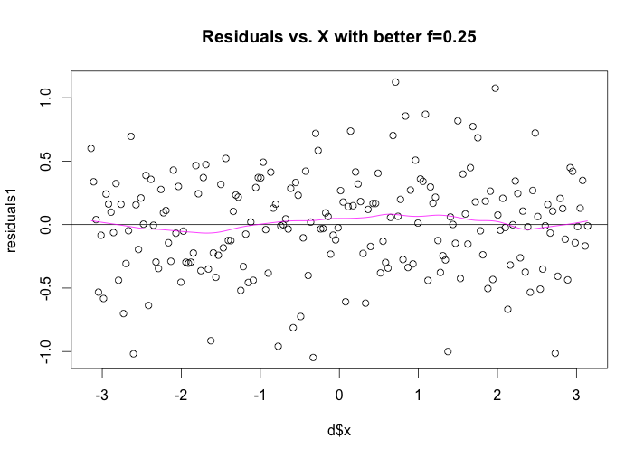

As we see in the above graph, comparing to the default value alpha=2/3, which has obvious fluctuate pattern in residual, the  loess curve on the residual graph is nearly a horizontal line and the residual graph has no certain pattern, with f=0.25, which means  the residuals is variation in y not explainable by x.

Also there is a new scatterplot of x and y, using a better choice of f.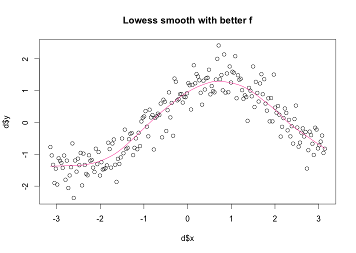

 

From the above graph, we can see that there is nonlinear relationship between x and y. An increase in Y as x increases until x is close to 1, the response is in fact constant until x=-2 and then the response increase as x increases until x=1. From 1 and above, the an decrease in Y as x increases until x is close to 3,saying a negative relationship between x and y. Comparing the first graph using default f, this lowess smooth explain the data better, telling us more detail information from the graph.

Finally, for better visual effect, I combine the scatterplot with lowess smooth and a plot of residual with lowess smooth in one graph. From the following graph, we can see that with the residual graph has no certain pattern, the scatterplot with lowess smooth could explain the original data better.Comparing to the default value(alpha=2/3), alpha=0.25 yield better lowess smooth. Also,by combining two graph together, we can see clearly both relationships of y and x and residuals and x, with the same horizontal scale.

This entry was posted on Friday, March 15th, 2013 at 6:42 pm and is filed under Uncategorized and You can follow any responses to this entry through the RSS 2.0 feed. You can leave a response, or trackback from your own site.