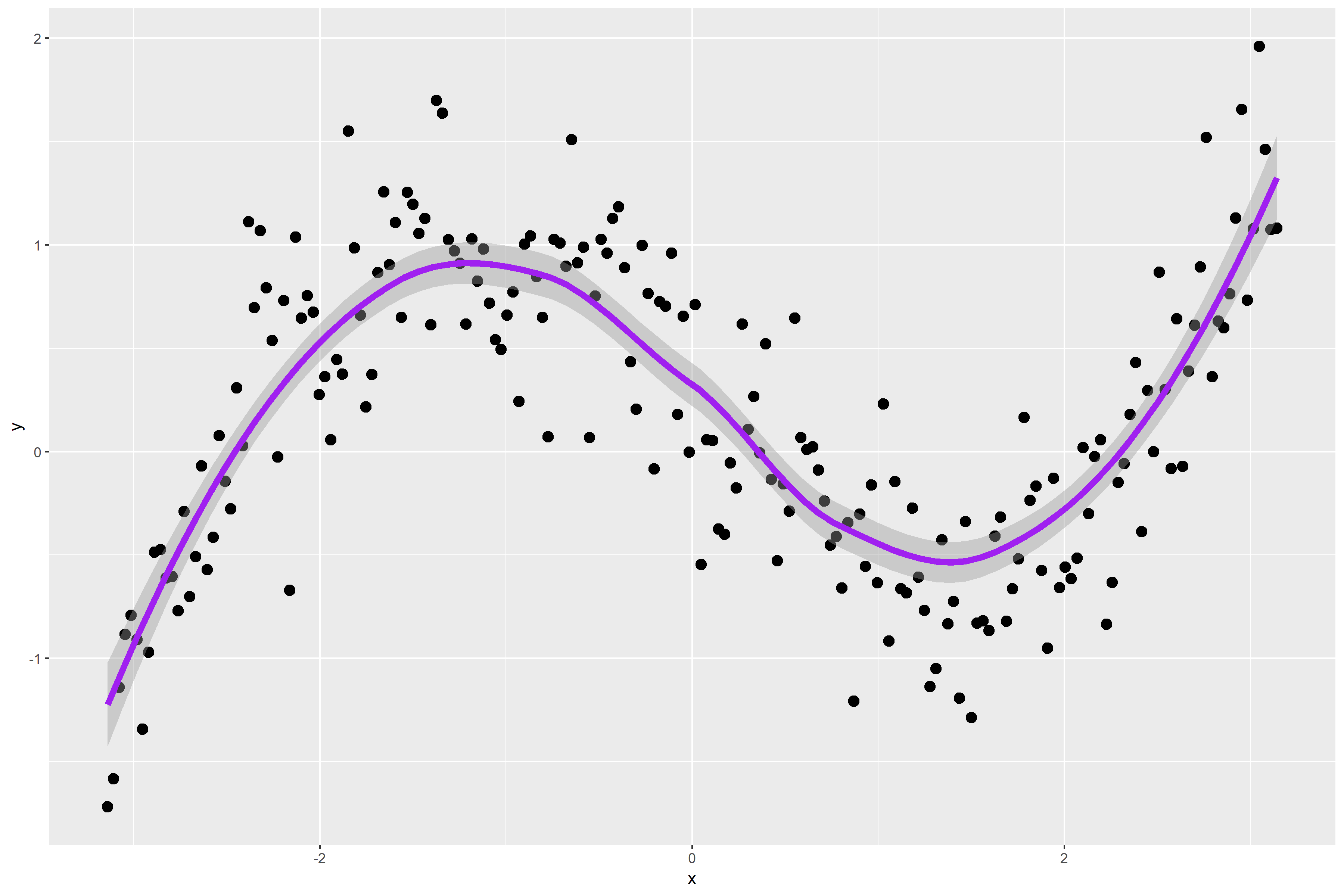
Figure 1. is a scatterplot of my randomly simulated data with a loess smooth overlay. The loess smooth overlay is set to its default value in ggplot2.

Figure 1.

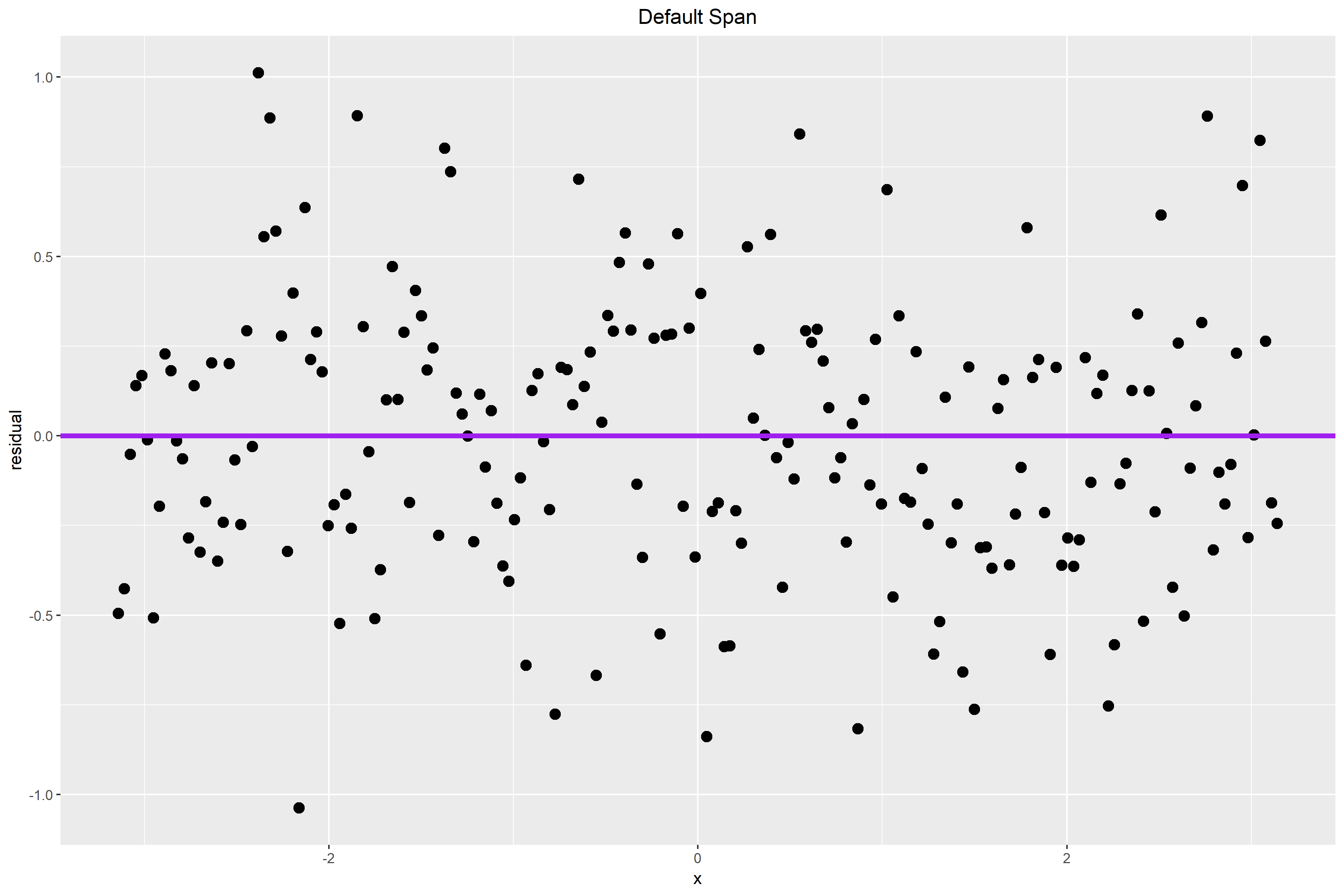
The following graph plots the residuals for my data points. The default span for the lowess curve appears to have found the signal fairly well. For the most part, the residuals are pretty randomly distributed. However, some may argue that there is a bit of a wave-like pattern in the residual plot.

Figure 2.

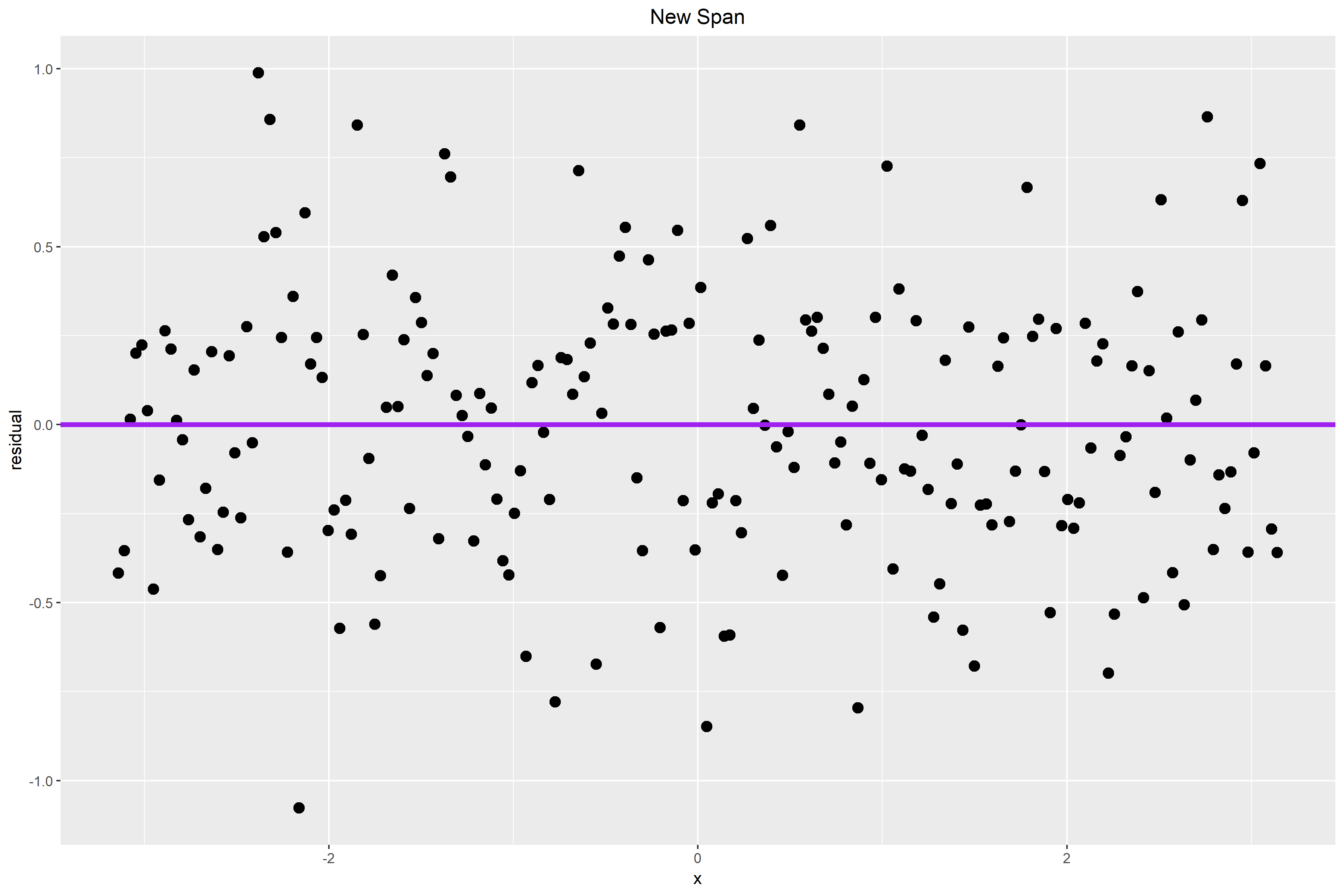
The plot below shows the residual plot after I changed the span from its default value to 0.65. The small pattern that we see in Figure 2. is probably caused by a larger alpha value. Therefore, I hope that by making alpha smaller, some of the pattern that we see in the residual plot above will be accounted for by the curve and new choice of the span.

In Figure 3. the residuals are closer to the horizontal line. The wave-like pattern that we see in Figure 2. also diminished slightly. The residuals appear to be more randomly distributed from before and there is less of a vertical spread. Thus, a span choice of 0.65 seems better than the default option.

Figure 3.

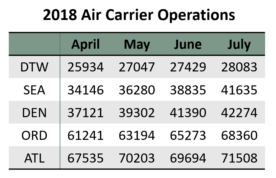
In this week’s blog assignment, I collected data on air carrier operations for five airports, namely DTW, SEA, DEN, ORD, and ATL. The response is the number of air carrier operations. The rows are classified by airports and the columns are classified by the four months between April to July 2018. The data is presented in the table below.

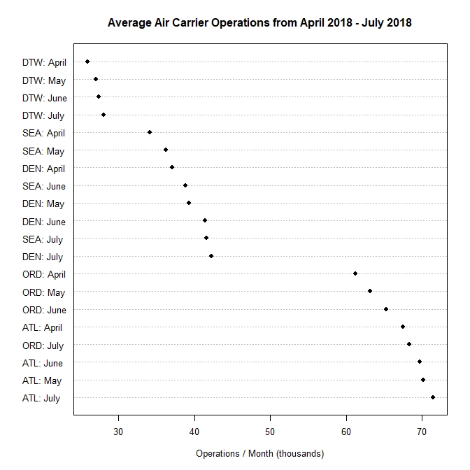
Figure 1. is a dot plot graphing the data. The horizontal scale measures the average number of air carrier operations in thousands. The vertical scale shows each airport and all four months. The mean number of operations is ordered from high to low as we read from left to right.

Figure 1.

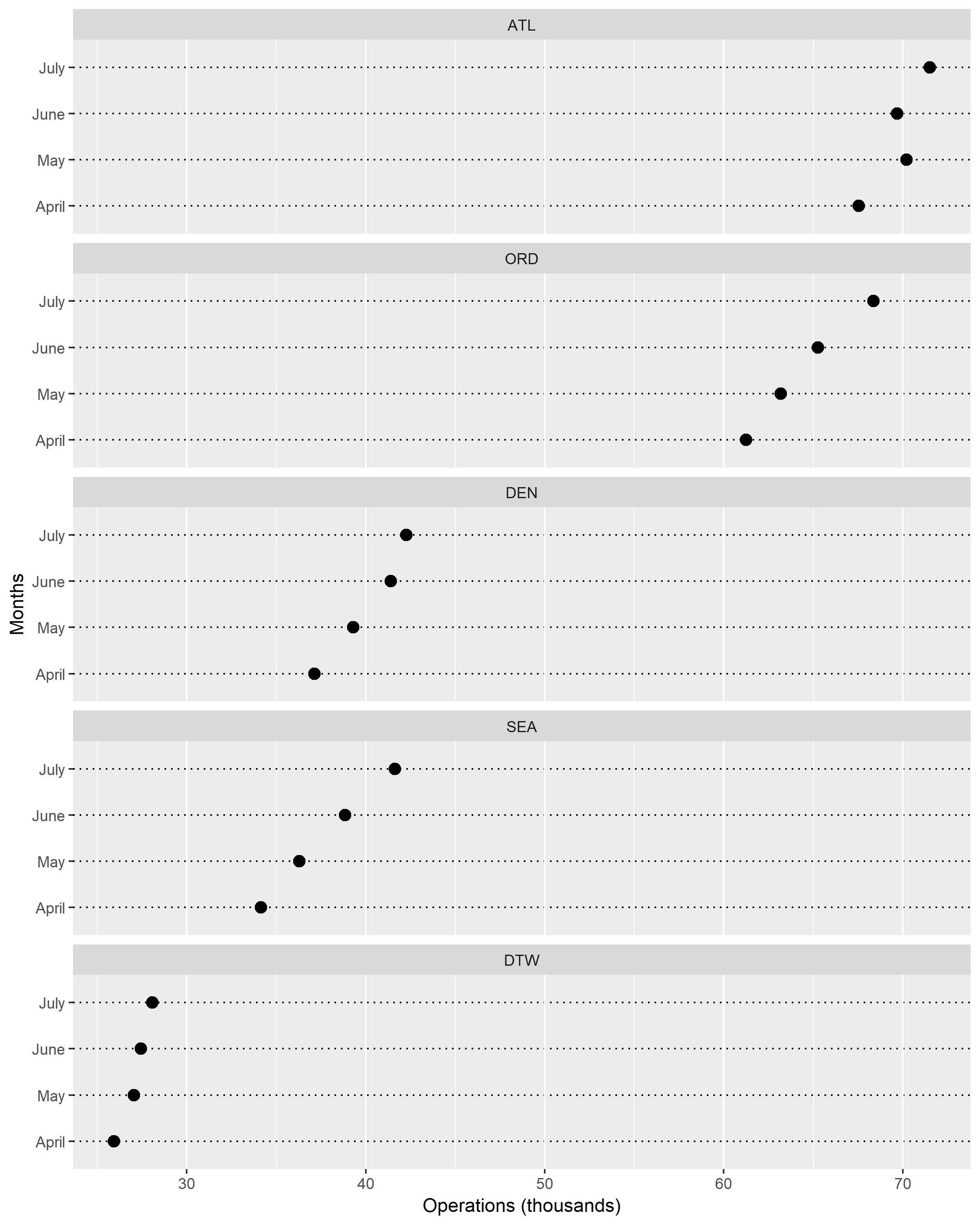
In Figure 2. I classified the multiway dot plot by rows. In this case, it was grouped by airports. I moved the panels so that it would show the airport with the largest number of operations at the top and smallest number of operations at the bottom. Clearly, we can see that there is a trend for each airport by month.

Figure 2.

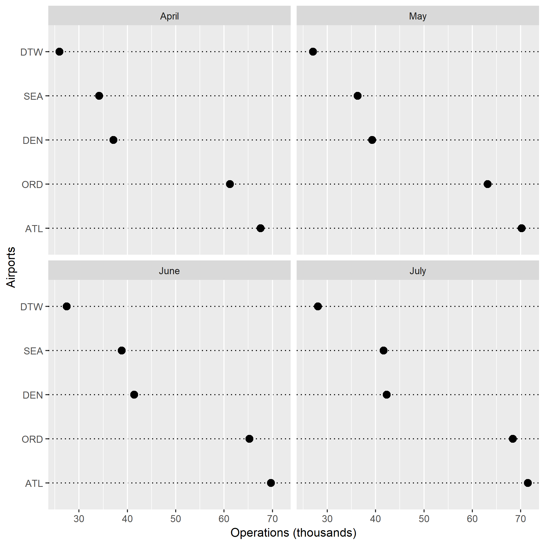
Figure 3. was grouped by columns, therefore by months. From this figure, it is also very clear that there is a trend for each airport. Throughout all four months, DTW has the smallest number of operations. In contrast, ATL remains as the airport with the most operations per month.

From these dot plots, I learned that the number of air carrier operations tend to increase as we move from the spring months into the summer months. This makes a lot of sense because more people are traveling during the summer, hence the jump in air traffic operations. The different types of dot plots that I generated taught me how each plot communicates information differently. Figure 1. gave me an overall glimpse at the trend of the data, but Figures 2. and 3. decoded the information in a more specific way. These two figures effectively graphed multiway data while retaining the labels.

I enjoyed grouping the data by rows (airports) more. Having all five panels on the same x-axis helped me to quickly and visually understand my data. Furthermore, grouping the data by airports just made more sense to me. I was able to look at the monthly trend and air carrier operations for each airport instead of looking at each month then comparing airports and their number of operations.

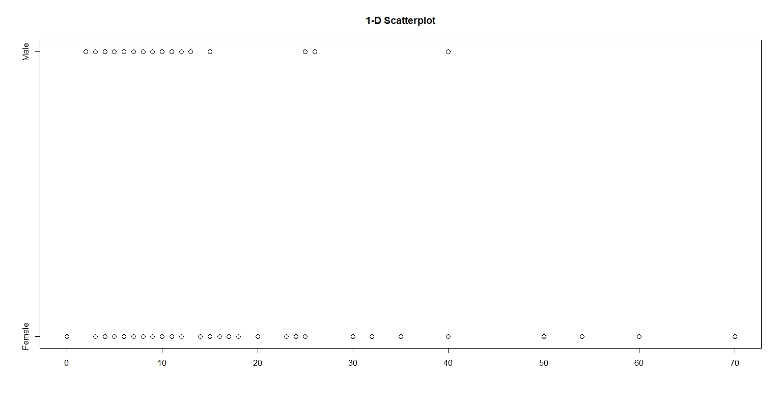
In this assignment, I examined the number of shoes owned by men and women in an introductory statistics class. Using the the package LearnBayes, I took a random sample of 100 from the dataset studentdata.  Figure 1. is a one-dimensional scatterplot with number of shoes on the horizontal scale. The vertical scale is categorized into two levels – male and female.

Figure 1.

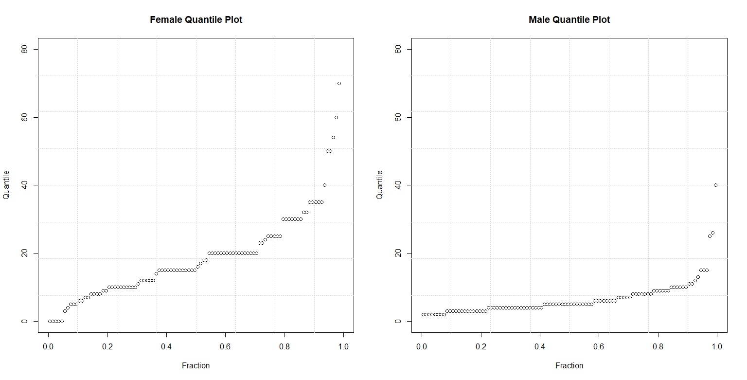
Figure 2. compares the quantile plots of the two gender and number of shoes. On each panel, the data is graphed against their respective f-values. On the left panel, we observe that the median number of shoes for women is almost 20. In contrast, we see on the right panel that the median number of shoes for men is short of ten. By looking at these parallel quantile plots, we can see that the median number of shoes owned by women doubles, more or less, that of men. Both quantile plots also reveal that the shape of the distribution of shoes is skewed. The majority number of shoes owned by males and females in this sample falls in the lower quartile, with a few in the upper quartile. Overall, the distribution of shoes for males and females is right-skewed with a few outliers near the 0.99 quartile.

Figure 2.

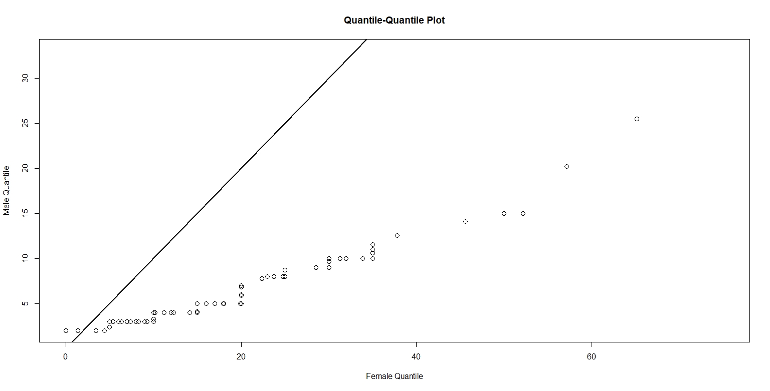
The following figure plots the quantiles of men against the corresponding quantiles of women.

Figure 3. 

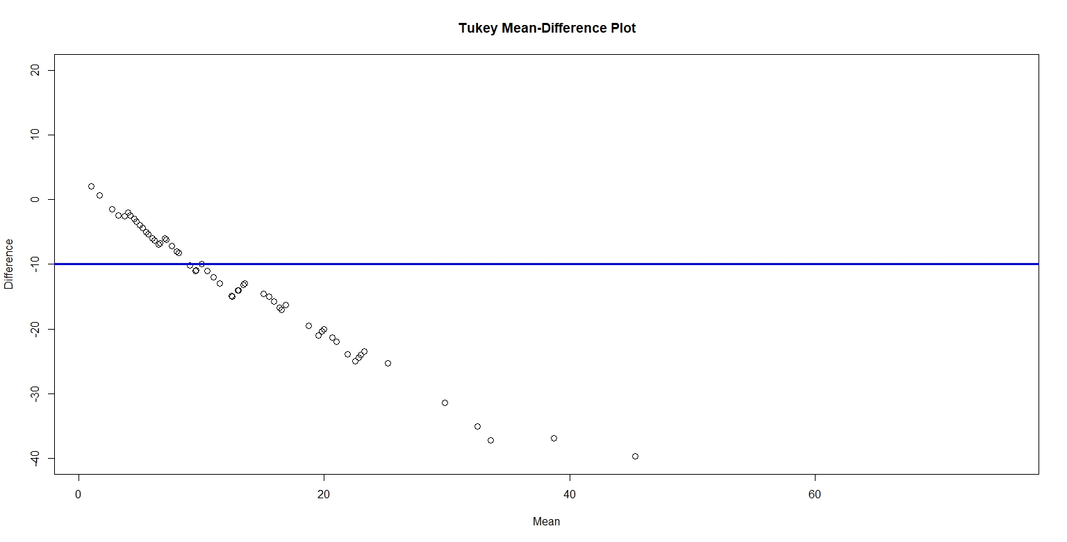
Figure 4. below plots the Tukey mean-difference for male and female number of shoes, with a horizontal reference line at -10. I chose to plot the horizontal line at -10 because the average of the difference is -10. The plot reveals that number of shoes for females is greater than men. On average, the increase in number of shoes for women is about 15. I believe the relationship between male and female values is pretty simple. That is, women tend to have more shoes than men.

Figure 4.

Between the four graphs, the Tukey Mean-Difference plot provides the best graphical comparison between the two sets. The Tukey Mean-Difference plot graphs the quantiles for the two sets together on one panel and lets us interpret the quantile difference on a horizontal line instead of a 45 degree diagonal line. Furthermore, we can easily and effectively compare the quantile differences to the average quantile. From this graph, we can deduce the number of shoes for men versus women. In short, the Tukey Mean-Difference plot is like a simple and meaningful summary of the other three graphs.

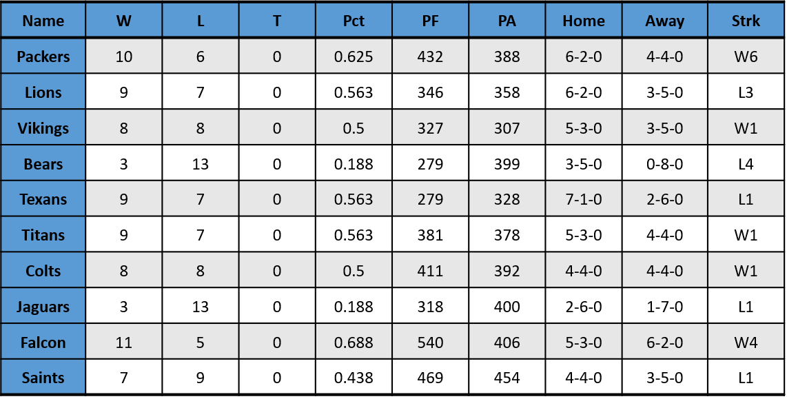
The data that I collected was based on the 2016 NFL Standings for 10 teams.  The data is provided in the table below, where PF (instead of P) represent “points for” the team.

Table 1.

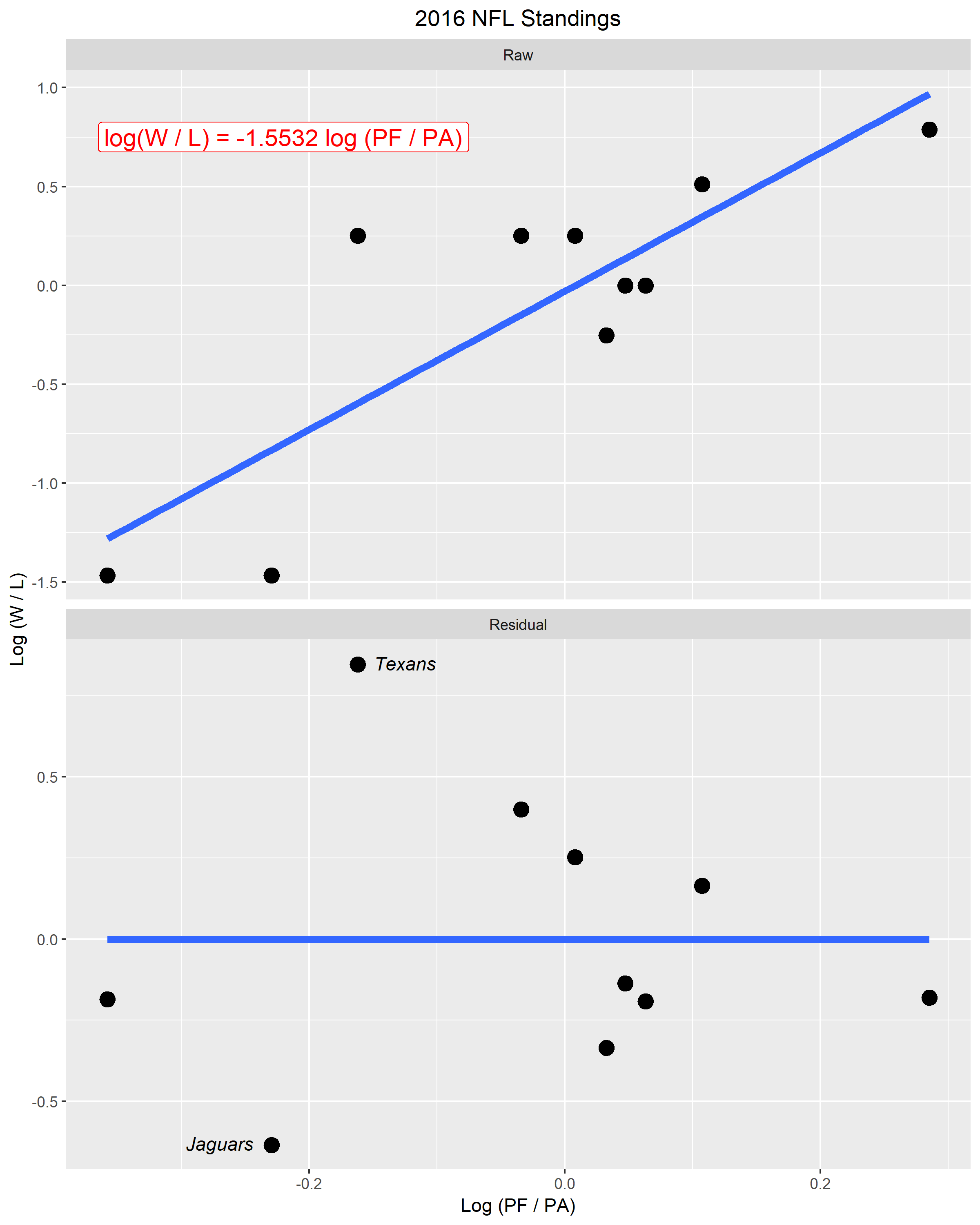
In the top panel of Figure 1., the horizontal scale measures the log ratio of total points scored for the team and total points scored against the team. The vertical scale graphs the log ratio of total wins and losses in the season. The best fitting line takes the form log (W / L) = k log (PF / PA), where k is taken to be -1.5532 in this particular data set.  I chose -1.5532 to be the ideal exponent because when (PF / PA) is taken to the power of -1.5532, it returned the closest values for number of wins. Additionally, the k that I chose fit the data best.

The bottom panel of Figure 1. is a plot of residuals against log (PF / PA). In this figure, I labeled two points that seemed “unusual” compared to the rest of the data. I identified these two “unusual” points by labeling them with their respective team names, Texans and Jaguars. These two points seemed “unusual” because their residuals were much greater compared to the rest of the data points. Furthermore, due to these two data points, the residual was not evenly distributed vertically.

Figure 1.