Figure 1. 
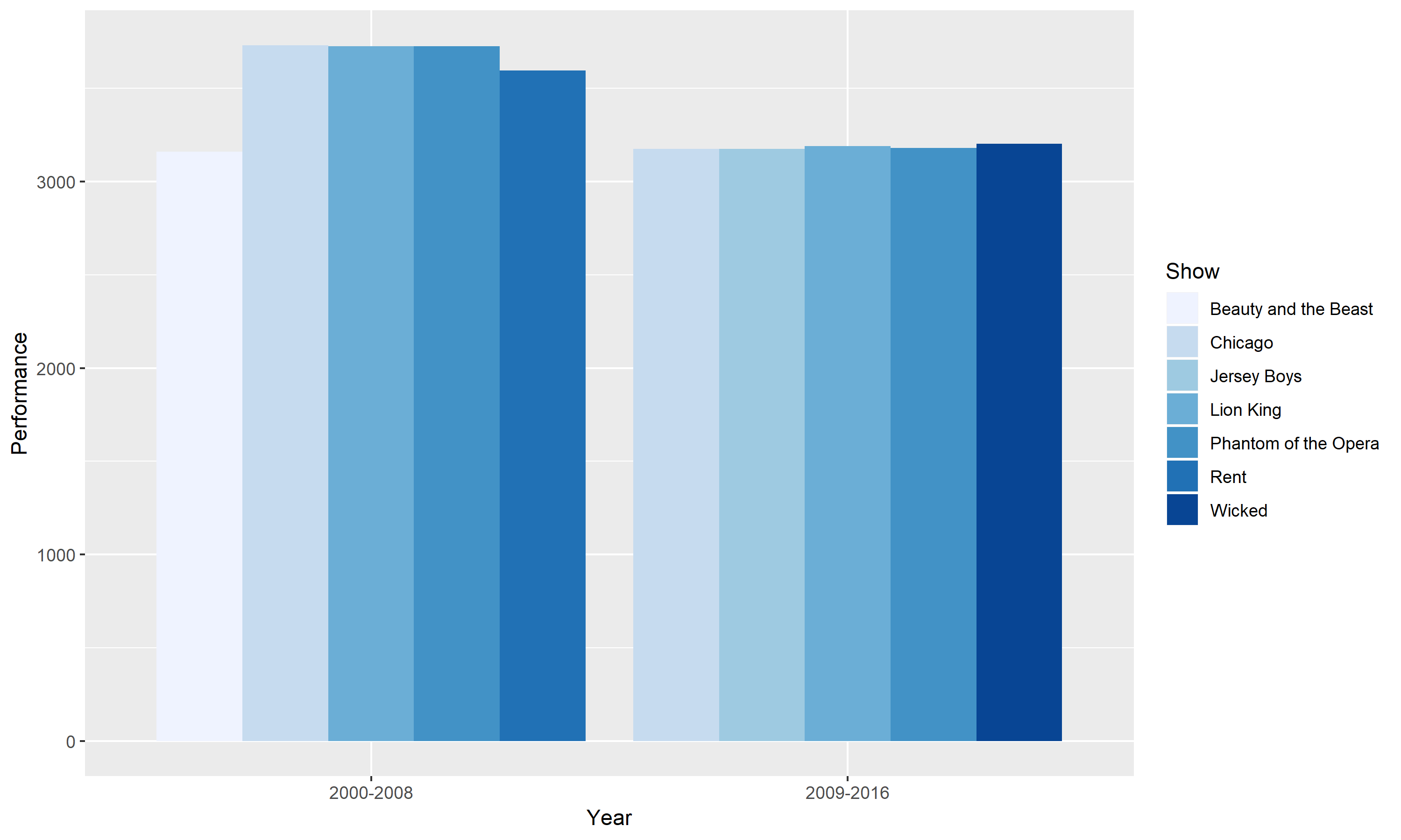
This graph compares the best Broadway shows for two time periods. The two time periods are between 2000 – 2008 and 2009 – 2016. The best Broadway shows are defined as having more than 3000 performances in each time range. The horizontal scale groups the two different period and the vertical axis shows the number of performances. From looking at this grouped bar chart, it is easy to identify that the 2000 – 2008 period had more performances. However, we also see an overlap of shows between the two periods. Chicago, Lion King and Phantom of the Opera appeared as three of the best Broadway shows for both periods.

Figure 2.
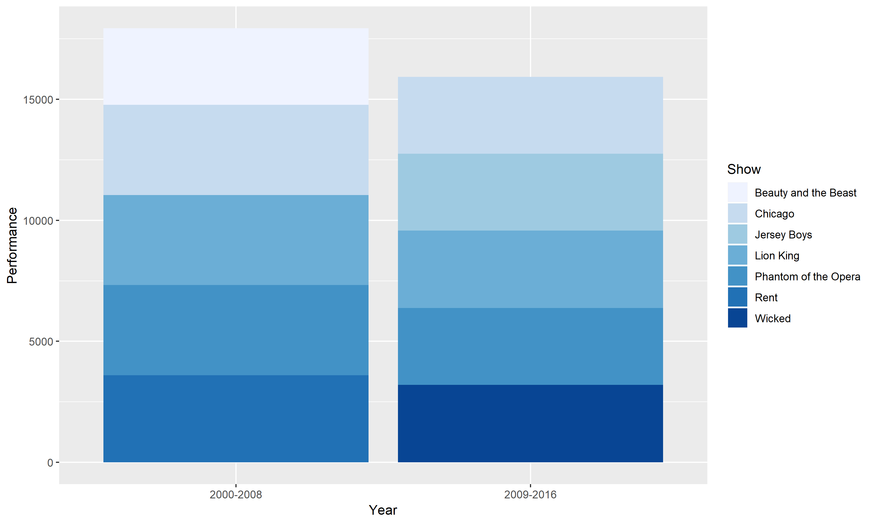
This chart is a stacked bar version of Figure 1. Instead of grouping the different shows, I stacked them on top of one another. The advantage to a stacked bar chart is it allows us to see how the best Broadway shows are divided into different show subcategories. However, a stacked bar chart may be harder to read especially when we want to compare each subcategory to another.

Figure 3.


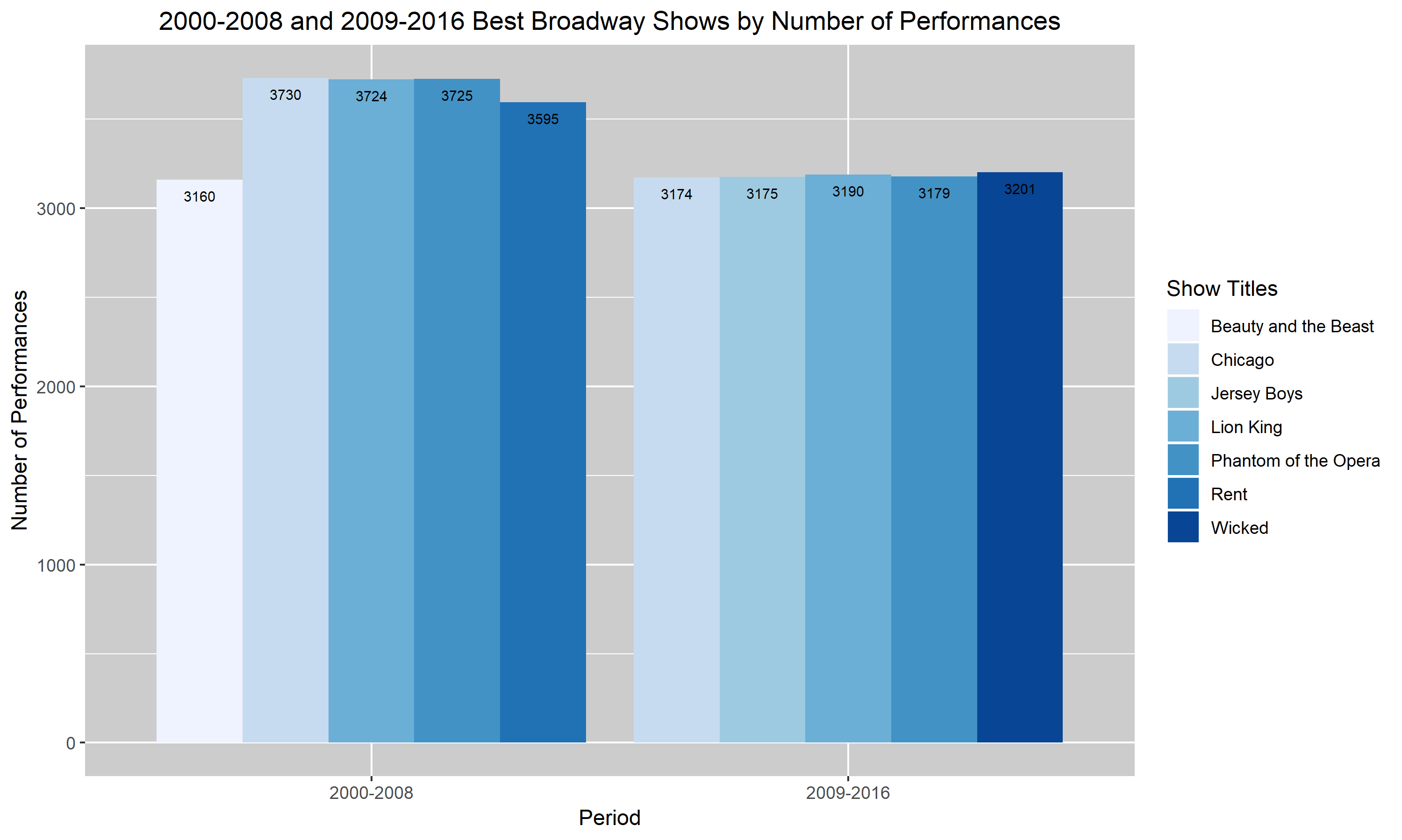
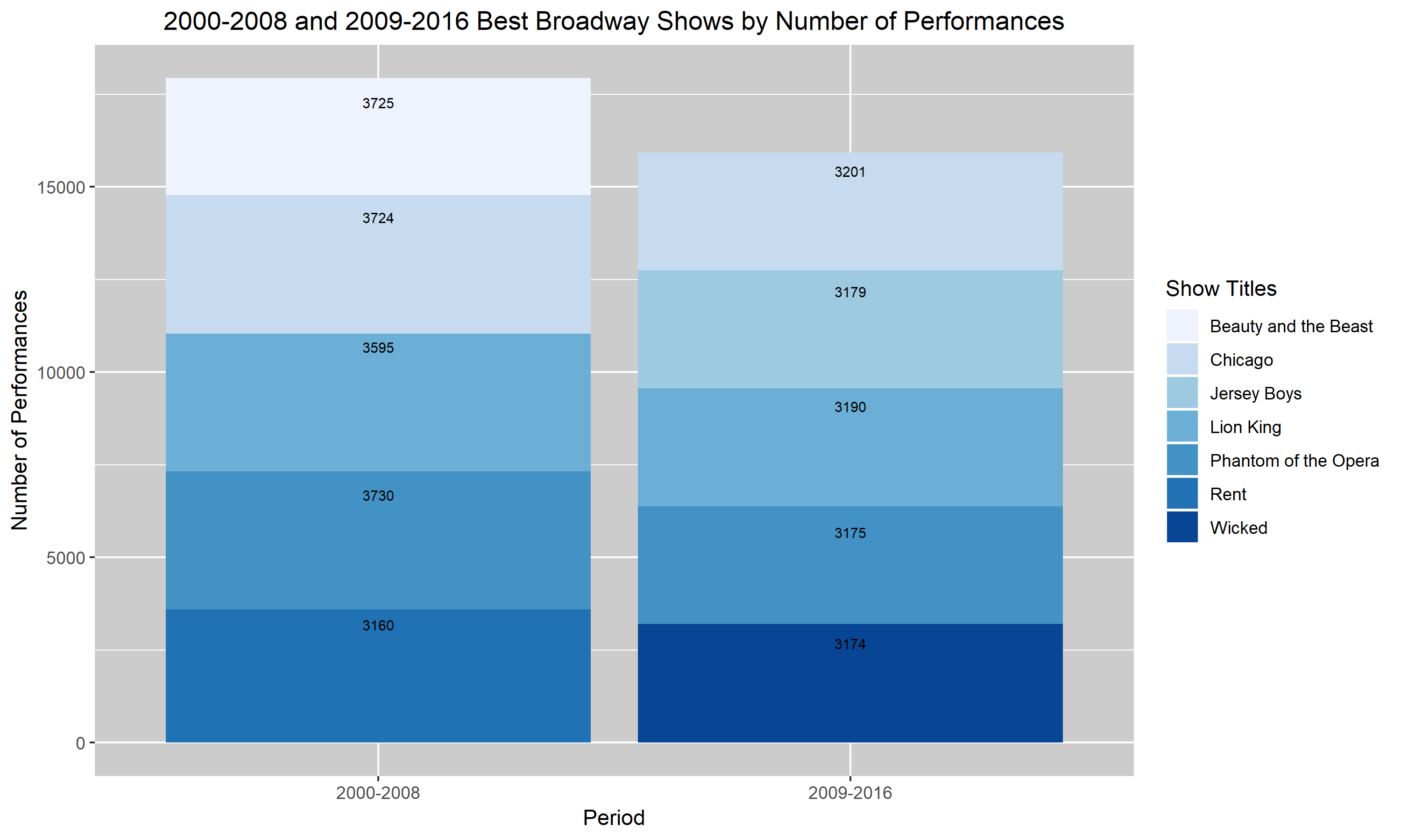
Figures 3. and 4. are my improved versions of Figures 1. and 2. I added a descriptive title to the figures so that my reader will have a rough idea of what my graph is trying to convey without having to read the caption. I also changed the labels to describe the scales more accurately. So, instead of saying “Year” and “Performances”, I changed it to “Period” and “Number of Performances”. Additionally, I darkened the background of my last two graphs. I realized that the very light blue bar in the first two graphs were almost hard to distinguish from the background. Hence, I darkened the background to help the bars pop up. Lastly, I added the values corresponding to each bar into my two final graphs. I felt like it was hard to compare each show and their number of performances in the top two graphs and so I decided that by having the values listed, it’ll help. Unfortunately for the darkest blue bar, the black font doesn’t pop up as well as I had hoped. I didn’t know how to choose a different color for that value specifically so I left it as is. I hope that with more research and assignments, I will learn how to distinguish that value through the use of color.

Figure 1.

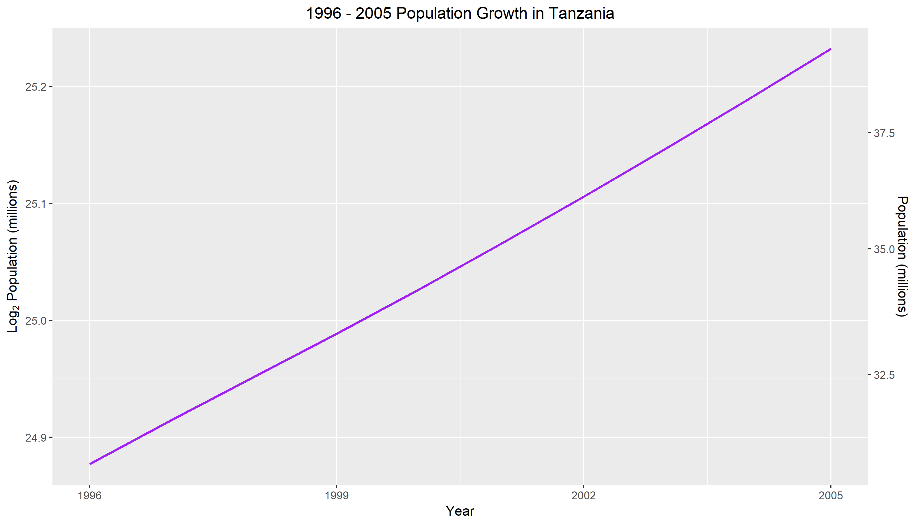
Figure 1. measures the population growth in Tanzania for a ten year frame. The horizontal scale is measured in years starting from 1996 to 2005. The left vertical axis uses a log base 2 scale and is measured in millions. The right vertical scale uses the original population units and is calculated in millions. From looking at the graph, we can see that there is an exponential relationship for population growth in Tanzania. That is, with each passing year, the population tends to increase. Comparing the year 1996 to 2005, we can see that the population has increased from less than 32.5 million to more than 37.5 million. Although the rate of change is minuscule, we can see that the slope is slowly getting steeper with each year.

Figure 2.

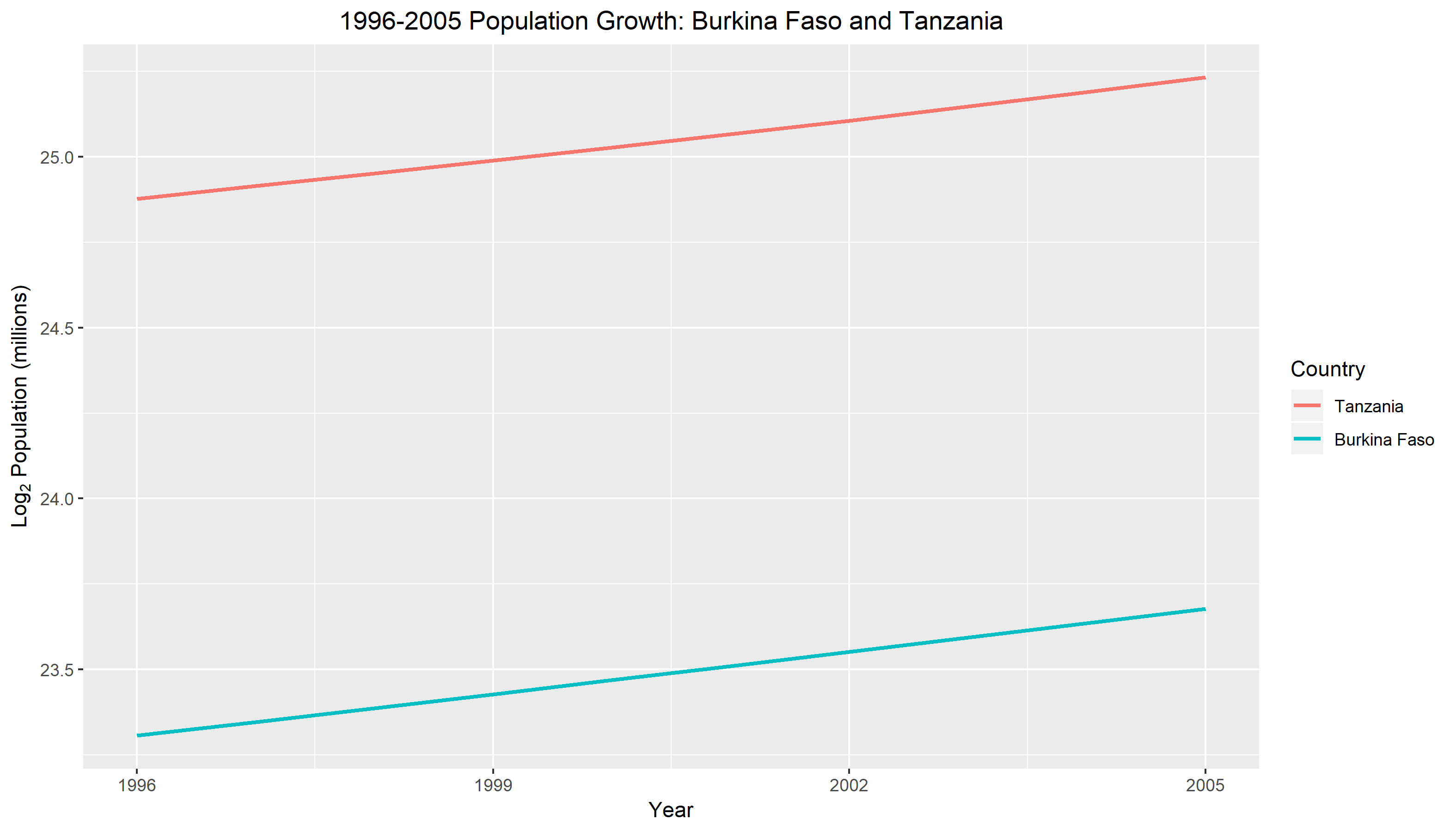
In Figure 2. we compare the log base 2 population growth against year for two countries. The two countries in this study are Burkina Faso and Tanzania. The horizontal scale is measured in years from 1996 to 2005. The vertical scale uses a log base 2 transformation and is given in millions. The graph reveals to us right away that Burkina Faso has a much smaller population size compared to Tanzania. This can be seen from the distance between the two connecting lines. Although their population sizes are different, both countries displays an exponential relationship between population and year. We can see from the graph that with each year that goes by, the population is increasing at a steady rate.

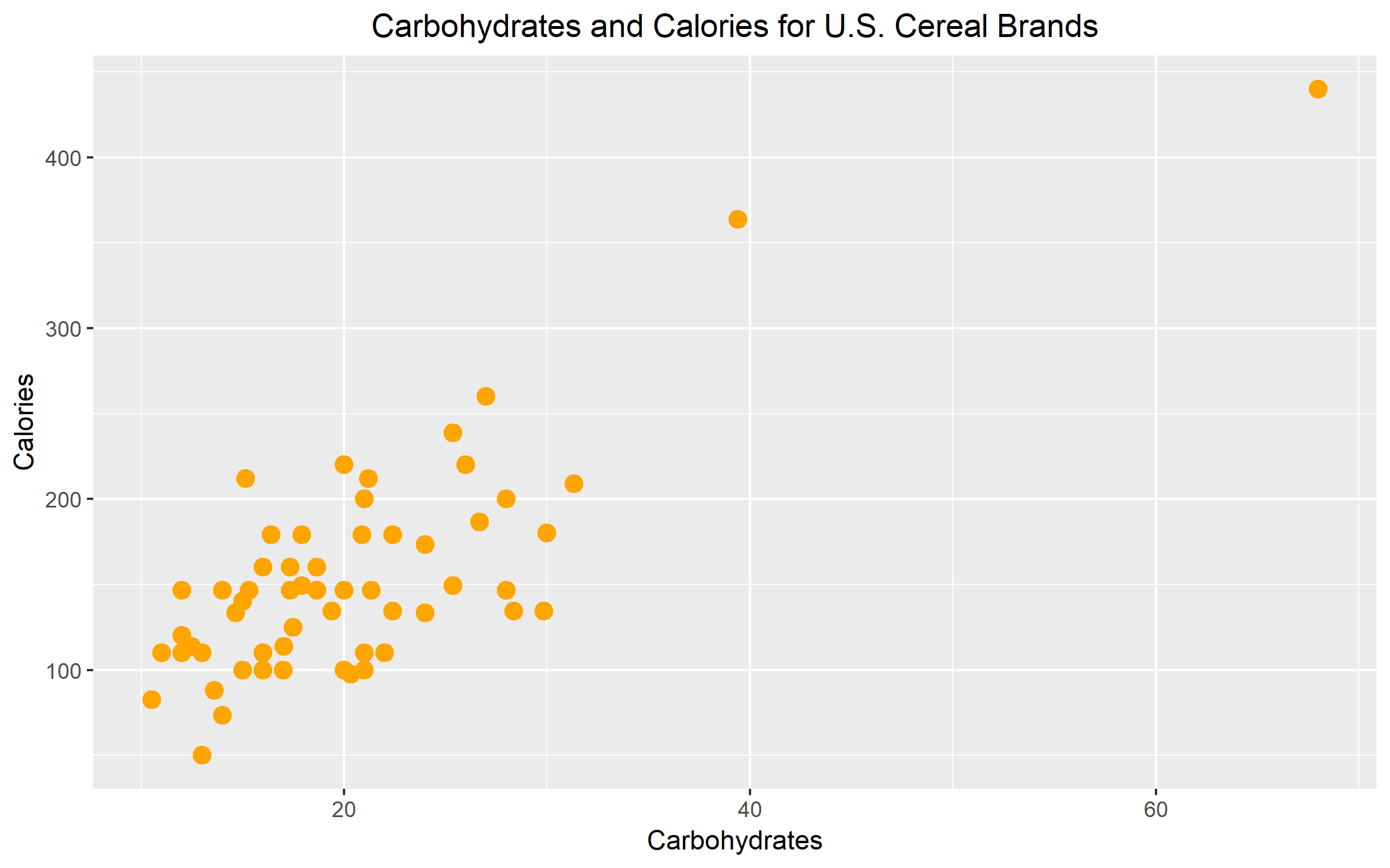
Figure 1.

 Figure 1 illustrates the nutritional relationship between carbohydrates and calories for a selection of U.S. cereal brands. The graph reveals a positive but moderately weak relationship between the carbohydrates and calories. The average carbohydrates for U.S. cereal brands ranges between 0 to 30. The average calorie count for U.S. cereal brands fall is between 0 to 250. The graph suggests that as the number of carbs increases, so does the number of calories.

Figure 2.

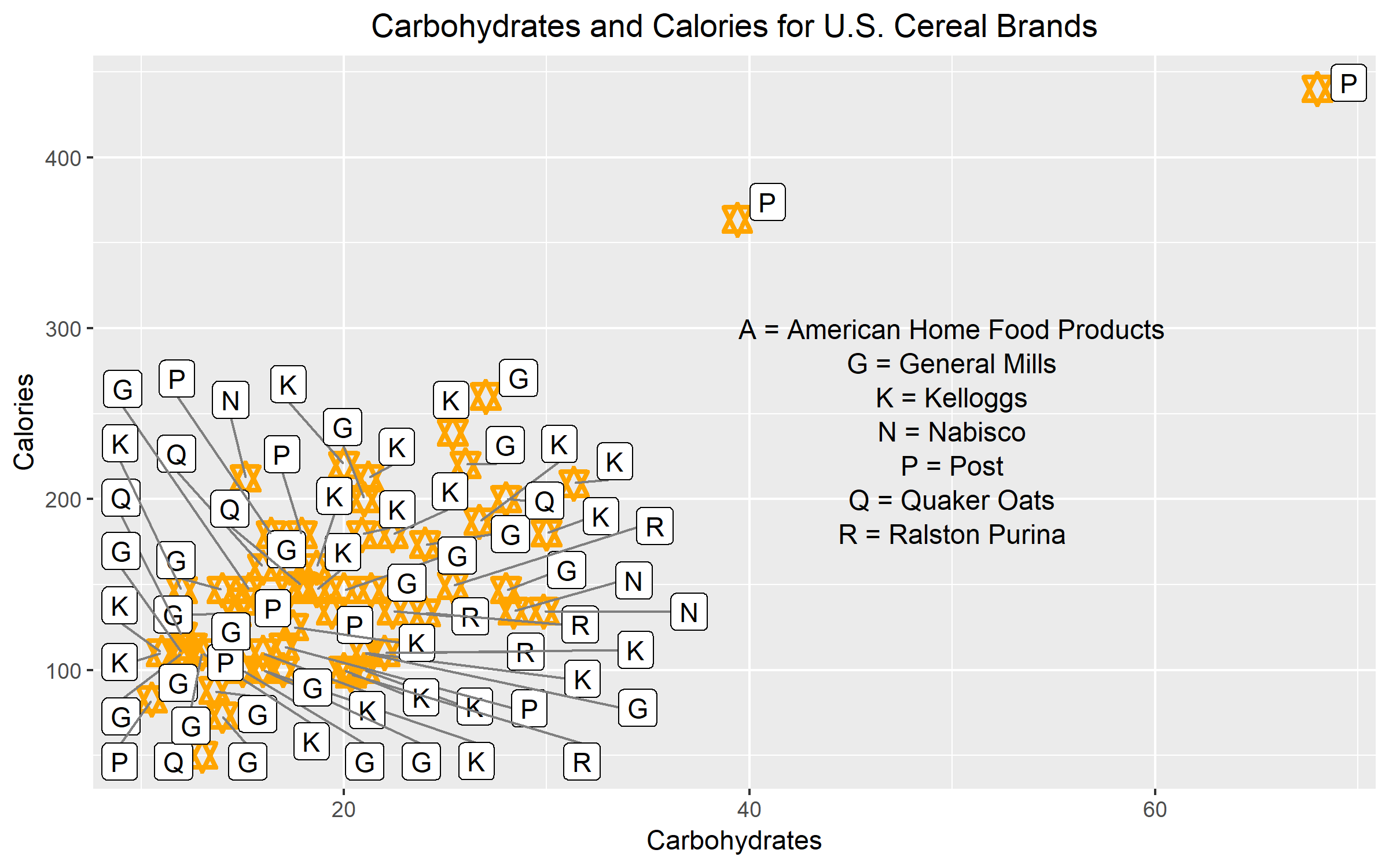
Figure 2 was redrawn from Figure 1. However, the graph was modified to violate at least two attributes of clear vision. The first modification leading to unclear vision was the use of data labels inside the scale-line rectangle. For each data point, I assigned the corresponding manufacturer label to it. As we can see, the label interferes with the data and clutters the graph. The key also adds to the graphical mess. The second modification that pushed this graph to have unclear vision was the graphical element. The plotting symbol that I used for this example was a star. The star is too fancy. The different points and lines of the stars are not prominent enough to stand out. It is hard to distinguish how many points make up the area where most of the data values are concentrated.

Figure 3.

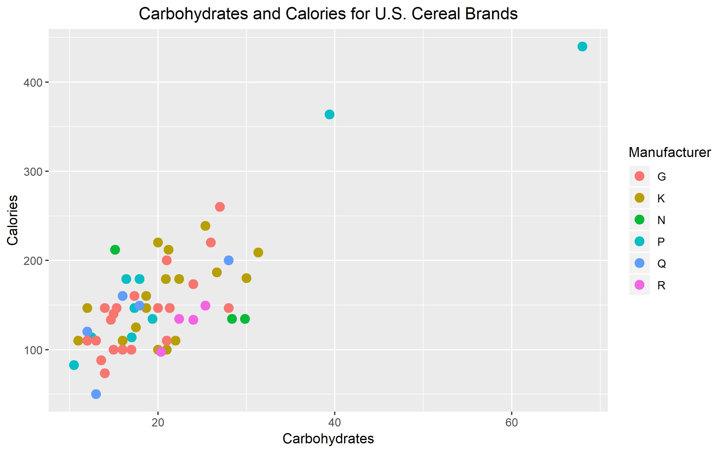
The third variable that I chose was the U.S. cereal manufacturer company. I chose manufacturer as my third variable because I believe that different companies may have their own set of regulations for nutrition. This can change how much calories and carbs are in each cereal box or serving size. Overall, I think that my graph is effective in representing my third variable. I think that between the three ways that could’ve been used to distinguish my third variable, color was definitely the most effective. I believe that color was effective because there are six different manufacturers. Using six different plotting symbols or six different sizes would make the graph look too messy. In the end, color was the best option. It worked out perfectly too because the pop of color makes it easy to identify the manufacturer for each data point.

Instructional fees per term at BGSU were collected for some selected years to assess the relationship between the two variables.

The scatter plot reveals a positive relationship between the two variables. We can see from the plot that as the years go by, instructional fees per term increases. The decade between 1980 and 1990 marks a time where fees increased the most rapidly.

The assignment provided some challenges. The hardest part for me was trying to figure out how to change the plotting symbol, how to thicken it and how to change the size of it. I wasn’t familiar with where to specify these aesthetics in my code and so I spent quite a bit of time returning error messages. After figuring how to customize the plotting symbol, I was able to thicken the connecting line with no trouble.