This week has provided a golden opportunity for me. Unlike past assignments involving familiar graphs and topics such as baseball and Broadway shows, this week’s assignment allows me to explore some unfamiliar territory. Truth be told, I have never used R to perform a loess smooth on a scatter plot. This week changed everything.
Let’s get started.
Loess Smooth on a Scatterplot
To achieve our x and y values for the initial scatterplot, I read a function into R Studio from the Canvas module. This function simulates some (x, y) data where the true signal follows one of the curves sin(x) + cos(x), sin(x) – cos(x), sin(x) * cos(x).
After reading in the simulated data, I plotted the points onto a scatterplot using ggplot under the Tidyverse R library. Subsequently, I overlaid a Loess smooth curve on the observations. For this figure, I used the default setting for span. This first figure is seen below:
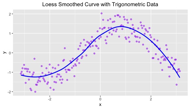
I am a big fan of the Loess smooth over this data. The observations follow a curve trend (understandably, since the read-in function is trigonometric), and a Loess curve perfectly captures this general trend.
To see if this curve is an acceptable fit, I plotted the residuals for this scatterplot. My hope was to see randomness exists in the residual plot. In addition, I included the trend line for the residuals. If the residuals are truly random, then the trend line should lie completely horizontal along the line y = 0.
Residual Plot
The residual plot is shown in the figure below. In this figure, the line y = 0 is green while the trend line is in blue.
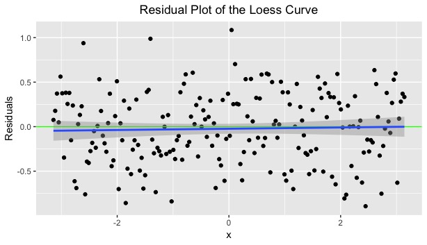
The residuals, at first glance, look to have no discernible pattern. This is a good thing! That must mean that the Loess smooth is a good fit for the data. However, the trend line is not perfectly horizontal; the slope is slightly positive. Thus, I deduced that there could be a possible Loess curve which more accurately represents the path of the x and y observations. The residuals provide strong evidence that the current Loess smooth is acceptable; however, it can be improved.
Loess Smooth (Span – 0.15)
In this next Loess smooth, I adjusted the span value of the function from its default setting to a value of 0.15. As a result, with a decreased span value, I anticipated the new curve to be less smooth. The result is seen below:
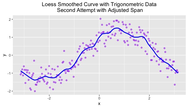
My premonition was correct in that the curve with the new span value is less smooth than the default curve. More prominent ridges are seen in this figure. However, I believe this figure is a better fit for the data since these ridges allow for the best-fitting line to become closer to the observations. To confirm this belief, I plotted a second residual chart, considering the new span value of 0.15.
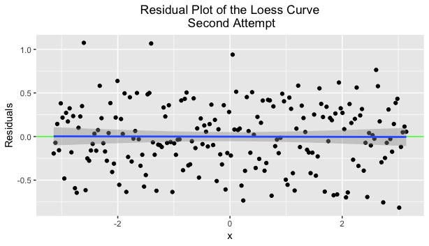
While it does not initially appear that the residuals are more or less random, the trendline allows the viewer to differentiate their values from the initial residuals. This trendline appears to be perfectly overlaid on the line y = 0; in other words, the trend line for the residuals is now completely horizontal. This means that the residuals are more random that the residuals from the previous curve. The adjusted span of 0.15 in the new Loess curve allows for more variability in the residuals; thus, the adjusted Loess smooth is a much better fit for the trigonometric data.
In this assignment, I discovered that changing the value of the span in the Loess function allows the function to become more or less smooth. As a result, the change in span also adjust the values of the residuals. In this particular study, the change in span allowed for a better fitting curve and more randomness in the residual plot.