In order to demonstrate that  “Any data that can be encoded by one of these pop charts (such as a pie chart, divided bar chart or an area chart) can also be decoded by either a dot plot or multiway dot plot that typically provides far more pattern perception and table look-up than the pop-chart encoding.”, I picked up two examples of pop charts.

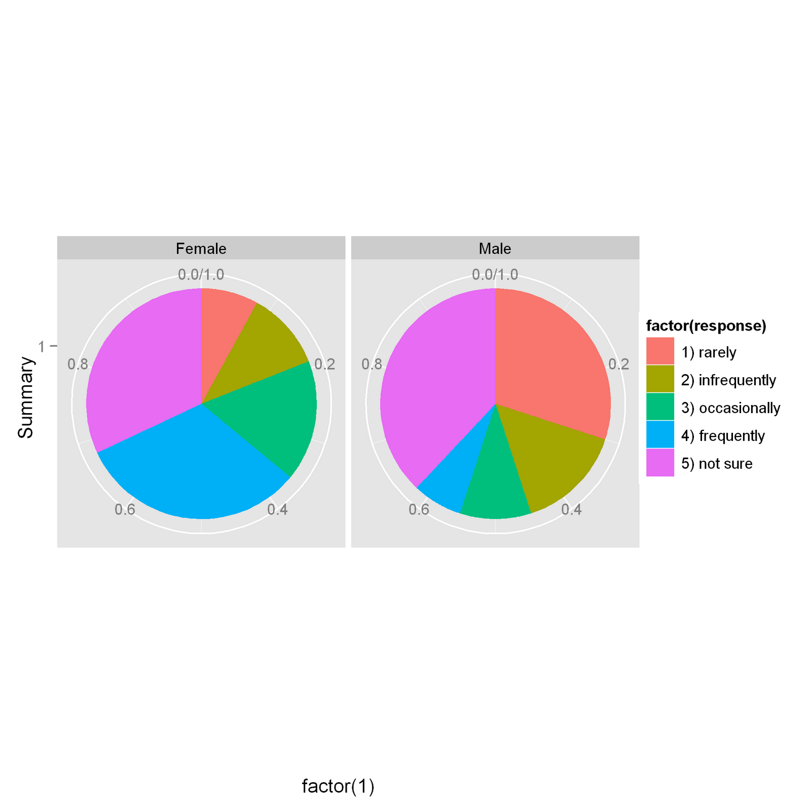
This pie chart gives an ordinary response of how frequently people would go shopping on weekends grouped by gender. One apparent drawback of this graph is that the quantitative side of the data is not easy to obtain. Also, the color encoding is not enough representative for the orders of the responses.

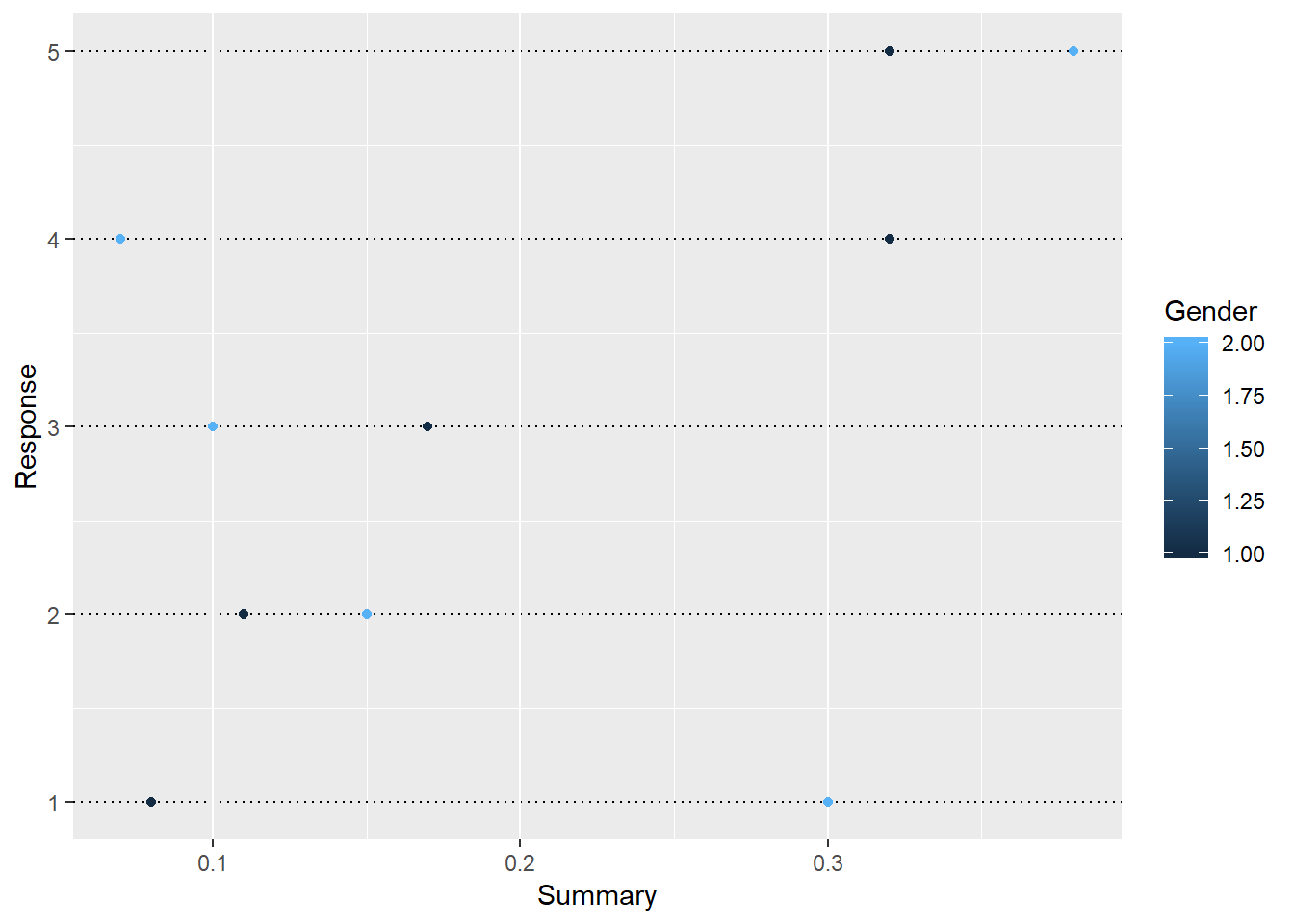
After transforming into a dot plot, these responses are listed in 5 rows. More importantly, for each response, we have clear impression of how the values can differ for males and females in dots with different colors.

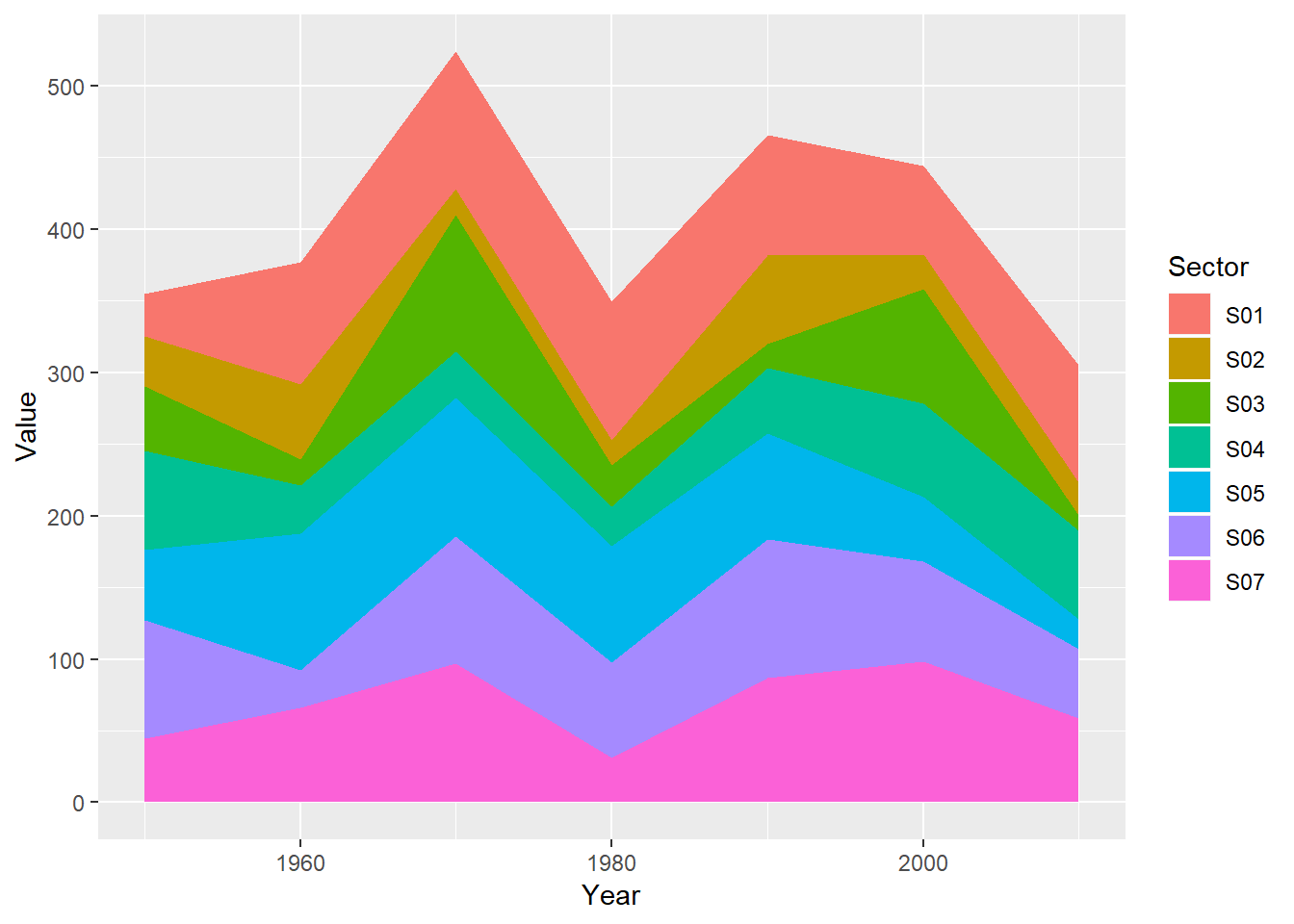
The second example is an area chart of seven groups. It has more or less the same issue as the first example which is not that reader-friendly for comparison and classification. Again, this encourages me to apply multiway dot plot for better interpretation of data as following.

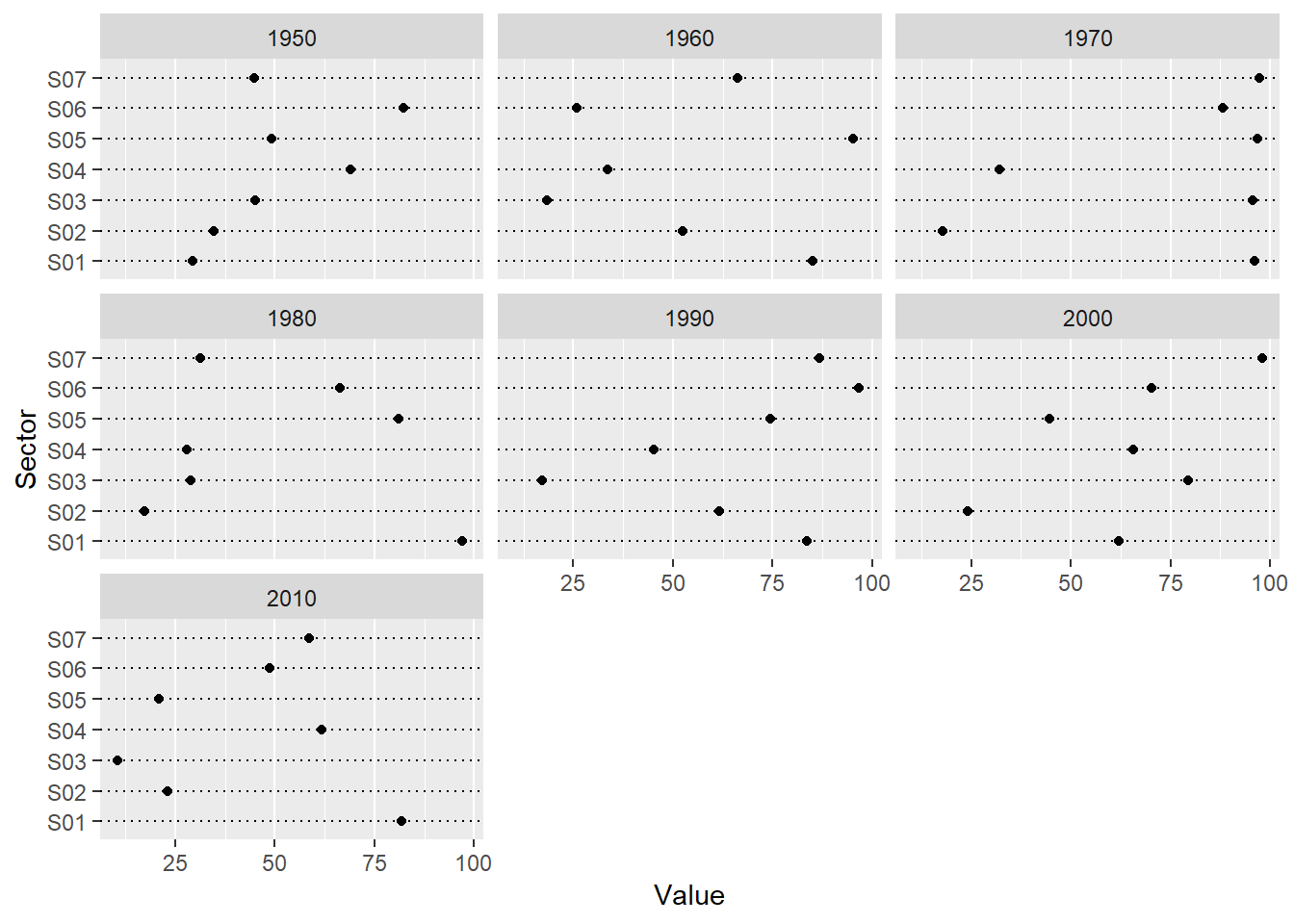
Now we seems to have more enough evidence to conclude which sector has the most or the least quantitative values in each year, and it’s relatively easier to actually obtain the values. Additionally, we have straightforward comparison among the years as well because these values share the same horizontal scale.

The dataset UScereal in the MASS package gives eleven variables for a group of 65 breakfast cereals.  I choose the variable calories, sodium and potassium to explore their general relationships using the scatterplot matrix, the  coplot, and the spinning 3-dimensional scatterplot below.

Scatterplot matrix:

There is a general positive trend between calories and sodium, cereals with higher calories tend to contain more sodium as well. And this positive correlation is even more solid with calories and potassium as dots stay closer to the smoothing despite the fact that there are three “special” types of cereals which are the “100% Bran”, “All-Bran with Extra Fiber”, and “All-Bran”(red dots) whose potassium is abnormally high at a relatively small calorie value . Also, cereals with higher sodium tend to contain more potassium.

Coplot:

As seem from the scatterplot matrix above, the values of sodium are quite constant and we seem to be more interested in the stronger correlation between calories and potassium so I construct this coplot of calories as a function of potassium given sodium. We’re supposed to observe a solid positive slope which is not always the case shown in this coplot since these three “special” cereals are quite off the trend.

Spinning 3-dimensional scatterplot:

The spinning feature helps us observe the 3-d structure of theses three variables. What we can see from this plot is that most observations do not stray far from the “diagonal” of the cube where all these three variables change in the same direction which verifies the fact that there are general positive trends between the calories, sodium and potassium.

The web page https://think.cs.vt.edu/corgis/csv/broadway/broadway.html provides an interesting dataset about Broadway shows.

I plot the time series plots on the graph blow about the Capacity(which is measured out of 100 percent) of the show “Jersey Boys” as a function of week numbers grouped by the year 2005-2016 with the smoothing.

What stands out in this plot is there is an apparent increasing trend at the year 2005 when the show released, and the decreasing trend since 2015 when the show were taken out of theater. Within our expectation, that show was hot from the year of 2006 to 2012 where the colors are closed to green.

Next I simulated a sample of size 200 from a bivariate normal distribution with correlation rho = -0.9 and use a bivariate density estimation algorithm to construct a contour graph of the density estimate.

And compared with the sample contour plot.

It not hard to find that the first graph better distinguishes the simulated data since it has a smaller amount of layers of colors within one theme from white to green whereas it becomes ambiguous to tell, especially for the light colors, in the second graph.